A/B testing: An online formula for Bayesian testing

I’ve developed an online formula for Bayesian A/B testing expanding Chris Stucchio’s and Evan Miller’s work.

Intro to A/B testing

A/B testing is a very natural and powerful tool for optimizing a website. Suppose you want your users to sign up for your newsletter. Your website’s call to action is “Sign up now!”. However, you wonder if maybe “Sign up today!” will be more effective. You show your version A website (“Sign up now!”) to some of your users; and create a version B (“Sign up today!”), shown to a second group of your users. The questions is: Do I leave my webpage as is (that is, keeping version A), or do I change it to version B?

In the Amazon developer webpage, we have this snippet.

Once you have chosen the metric you care about (in our case, clicking the button), we estimate the “conversion rates” for group A and B, p_A and p_B respectively, where p_A = (number of conversions in group A) / (size of group A), and p_B = (number of conversions in group B) / (size of group B). Bear in mind these are mere estimates of the true, unknown conversion rates. Our previous questions becomes: What is the probability of p_B being greater than p_A, or, Prob(p_B > p_A) ? Of course, we cannot ask every single person of the planet to choose. Also, a single person’s decision of clicking our button may change from one day to another. That is why we rely on experiments and statistics. The most straightforward statistical test to perform is a z-test, as explained in the Amazon developer webpage. Certainly, for large enough samples (over 1000 views, says this source), this is a good approach. However, what happens if our sample size is way smaller than that? Or, if we are required to end our A/B test early?

Bayesian statistics

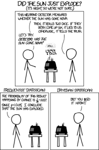
This is where Bayesian statistics come to the rescue. Bayesian methods allow us to incorporate prior information or beliefs into our models, allowing us to make a more informed decision. Or, as the xkcd comics describe it:

Bayesian A/B testing

I first started learning about A/B testing from Chris Stucchio’s blog. In it, he very intuitively describes Bayesian A/B testing and gives access to some python code for numerically computing the quantities of interest, namely, a double integral. We can see the mathematical derivation of this in this great post by Evan Miller, as well as a closed-form solution for it. Basically, we say the conversion rates have a prior distribution of a beta distribution. Afterwards, Prob(p_B > p_A) is computed as the double integral of the joint distribution of p_A and p_B (which, given independence, is just the product of the individual distributions) where p_B > p_A. This yields the beautiful closed-form solution:

Moreover, Evan Miller derived the following equivalent equations.

Here is some python code I wrote that calculates Prob(p_B > p_A).

def bayesian_test(alpha_A, beta_A, alpha_B, beta_B):
   prob_pB_greater_than_pA = 0
   for i in range(0, alpha_B):
      prob_pB_greater_than_pA += exp(log(beta(alpha_A + i, beta_B + beta_A)) - \
log(beta_B + i) - log(beta(1 + i, beta_B)) - log(beta(alpha_A, beta_A)))
 return prob_pB_greater_than_pA

from scipy.special import beta
from math import log, exp

alpha_A, beta_A, alpha_B, beta_B = 205, 104, 333, 273 
prob_pb_greter_than_pA = bayesian_test(alpha_A, beta_A, alpha_B, beta_B)

A note of caution: The beta function B(x,y) takes values very close to zero as x and y increase. For example, B(100,100) is 2.2087606931994364e-61. The log function in numpy handles these cases by returning an object, hence our using the log function in the library math instead. Also, to prevent numerical underflow, we take the logarithm of the expression and the exponential of it afterwards.

The online formula

It’s expensive to apply the beta function, logarithms and exponentials. We would like to apply these as little as possible. Notice how, for every new costumer in our A/B testing, first we decide to show version A or B, and then we record whether the costumer converted or not. This means only one of the four quantities    changes, the rest remain the same. And, the quantity that changes only increases by 1. For example, suppose the (N+1)-th costumer is shown version B, and he converts. That is,  changes, or,   , we then have:

We

now present the update formula for the three remaining cases. If    changes:

If    changes:

and, the last case, if  changes:

Finally, to initialize the algorithm, notice how  are all 1 for N=0. This yields the initial probability Prob(p_B > p_A) to be

The code

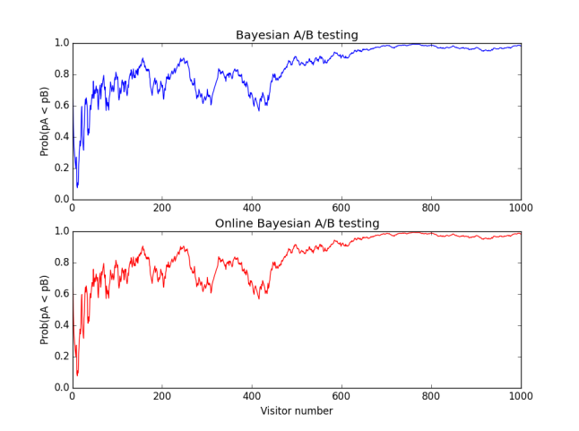
I wrote a python script implementing the online formula for Bayesian testing, and compare it against the original formula. You can find this code in my github account. Here is a plot of the output of my code, simulating an A/B test. One thousand visitors were shown version A or version B with equal probability. Afterwards, visitors shown version A would convert with probability 0.2 and those shown version B with probability 0.24. Here is the evolution of the quantity  Prob(p_B > p_A): Playing around with different values of pA and pB can give more insight into the problem. Finally, bear in mind that the beta function will numerically evaluate to 0 in values in the order of thousands. Thank you for reading!